โครงการอบรมเช งปฏ บ ต การ น กว ทยาการข อม ลภาคร ฐ (Government Data Scientist)
|
|
|
- Naomi Dennis
- 5 years ago
- Views:
Transcription
 (ว นท 2) สถาบ นพ ฒนาบ คลากรด านด จ ท ลภาคร ฐ สาน กงานพ ฒนาร")

1 โครงการอบรมเช งปฏ บ ต การ น กว ทยาการข อม ลภาคร ฐ (Government Data Scientist) (ว นท 2) สถาบ นพ ฒนาบ คลากรด านด จ ท ลภาคร ฐ สาน กงานพ ฒนาร ฐบาลด จ ท ล (องค การมหาชน) บรรยายโดย ผศ.ดร.โษฑศ ร ตต ธรรมบ ษด อาจารย ประจากล มสาขาว ชาเทคโนโลย การจ ดการระบบสารสนเทศ คณะว ศวกรรมศาสตร มหาว ทยาล ยมห ดล

2 2 Keep in touch Materials
3 3 Agenda Day [M07] Introduction to Machine Learning [M08] Basic Classification Techniques [M09] Classification Evaluation Techniques [M10] Regression Methods [M11] Advanced Classification Techniques [M12] Model Integration and Results Optimization
4 4 Agenda Day [M13] Advanced Data Preprocessing [M14] Clustering Techniques [M15] Semi-supervised Learning [M16] Association Rules Discovery
5 5 Agenda Day [M17] Introduction to Data Visualization and Business Intelligence [M18] Data Blending and Data Integration for Visualization [M19] Customizing Data Display [M20] Creating and applying predefined functions [M21] Visual Analytics, Dashboard Design, and Story Telling
6 6 Agenda Project Presentation Champion Announcement Day 5 (Pitching Day)
7 7 Module 7 Introduction to Machine Learning

8 8 What is machine learning? Machine learning is the subfield of computer science that, according to Arthur Samuel in 1959, gives "computers the ability to learn without being explicitly programmed. Evolved from the study of pattern recognition and computational learning theory in artificial intelligence, machine learning explores the study and construction of algorithms that can learn from and make predictions on data.
9 9
10 10 How Machine Learning Works
11 11 Module 8 Basic Classification Techniques
12 12 Classification: Definition Given a collection of records (training set ) Each record contains a set of attributes, one of the attributes is the class. Find a model for class attribute as a function of the values of other attributes. Goal: previously unseen records should be assigned a class as accurately as possible. A test set is used to determine the accuracy of the model. Usually, the given data set is divided into training and test sets, with training set used to build the model and test set used to validate it.
13 Illustrating Classification Task Tid Attrib1 Attrib2 Attrib3 Class 1 Yes Large 125K No 2 No Medium 100K No 3 No Small 70K No 4 Yes Medium 120K No 5 No Large 95K Yes 6 No Medium 60K No 7 Yes Large 220K No 8 No Small 85K Yes 9 No Medium 75K No 10 No Small 90K Yes Training Set Tid Attrib1 Attrib2 Attrib3 Class 11 No Small 55K? 12 Yes Medium 80K? 13 Yes Large 110K? 14 No Small 95K? 15 No Large 67K? Test Set Induction Deduction Learning algorithm Learn Model Apply Model Model

14 14 Classification Workflow (Basic)
15 15 Classification Techniques Decision Tree based Methods Memory based reasoning Naïve Bayes and Bayesian Belief Networks Neural Networks Etc..

16 16 Decision Tree

17 17 Decision Tree
18 18 Constructing decision trees Strategy: top down Recursive divide-and-conquer fashion First: select attribute for root node Create branch for each possible attribute value Then: split instances into subsets One for each branch extending from the node Finally: repeat recursively for each branch, using only instances that reach the branch Stop if all instances have the same class
19 19 Which attribute to select?

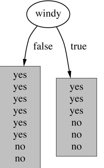
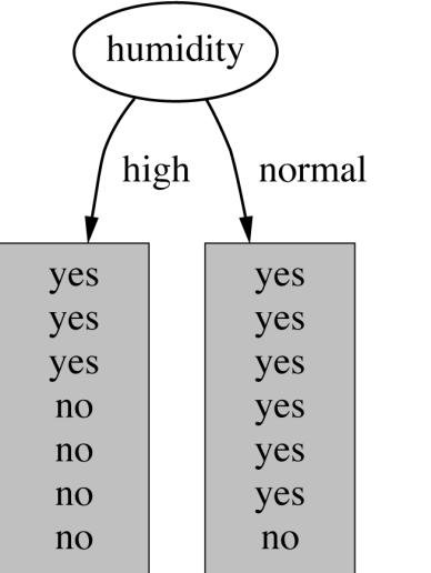
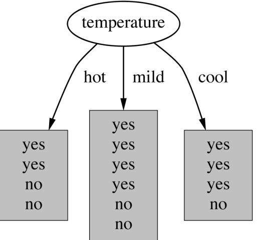
20 20 Which attribute to select?
21 10 21 Example of a Decision Tree Splitting Attributes Tid Refund Marital Status Taxable Income Cheat 1 Yes Single 125K No 2 No Married 100K No Yes Refund No 3 No Single 70K No 4 Yes Married 120K No 5 No Divorced 95K Yes 6 No Married 60K No 7 Yes Divorced 220K No NO MarSt Single, Divorced TaxInc < 80K > 80K Married NO 8 No Single 85K Yes 9 No Married 75K No NO YES 10 No Single 90K Yes Training Data Model: Decision Tree
22 10 22 Another Example of Decision Tree Married MarSt Single, Divorced Tid Refund Marital Status Taxable Income 1 Yes Single 125K No 2 No Married 100K No 3 No Single 70K No Cheat NO Yes NO Refund No TaxInc < 80K > 80K 4 Yes Married 120K No 5 No Divorced 95K Yes NO YES 6 No Married 60K No 7 Yes Divorced 220K No 8 No Single 85K Yes 9 No Married 75K No There could be more than one tree that fits the same data! 10 No Single 90K Yes
23 10 23 Apply Model to Test Data Start from the root of tree. Test Data Refund Marital Status Taxable Income Cheat Refund No Married 80K? Yes No NO Single, Divorced MarSt Married TaxInc < 80K > 80K NO NO YES
24 10 24 Apply Model to Test Data Test Data Refund Marital Status Taxable Income Cheat Yes Refund No No Married 80K? NO Single, Divorced MarSt Married TaxInc < 80K > 80K NO NO YES
25 10 25 Apply Model to Test Data Test Data Refund Marital Status Taxable Income Cheat Yes Refund No No Married 80K? NO Single, Divorced MarSt Married TaxInc < 80K > 80K NO NO YES
26 10 26 Apply Model to Test Data Test Data Refund Marital Status Taxable Income Cheat Yes Refund No No Married 80K? NO Single, Divorced MarSt Married TaxInc < 80K > 80K NO NO YES
27 10 27 Apply Model to Test Data Test Data Refund Marital Status Taxable Income Cheat Yes Refund No No Married 80K? NO Single, Divorced MarSt Married TaxInc < 80K > 80K NO NO YES
28 Decision Tree Classification Task Tid Attrib1 Attrib2 Attrib3 Class 1 Yes Large 125K No 2 No Medium 100K No 3 No Small 70K No 4 Yes Medium 120K No 5 No Large 95K Yes 6 No Medium 60K No 7 Yes Large 220K No 8 No Small 85K Yes 9 No Medium 75K No 10 No Small 90K Yes Training Set Tid Attrib1 Attrib2 Attrib3 Class 11 No Small 55K? 12 Yes Medium 80K? 13 Yes Large 110K? 14 No Small 95K? 15 No Large 67K? Test Set Induction Deduction Tree Induction algorithm Learn Model Apply Model Model Decision Tree
29 29 Tree Induction Greedy strategy. Split the records based on an attribute test that optimizes certain criterion. Issues Determine how to split the records How to specify the attribute test condition? How to determine the best split? Determine when to stop splitting
30 30 How to Specify Test Condition? Depends on attribute types Nominal Ordinal Continuous Depends on number of ways to split 2-way split Multi-way split
31 31 Splitting Based on Nominal Attributes Multi-way split: Use as many partitions as distinct values. Family CarType Sports Luxury Binary split: Divides values into two subsets. Need to find optimal partitioning. {Sports, Luxury} CarType {Family} OR {Family, Luxury} CarType {Sports}
32 32 Splitting Based on Ordinal Attributes Multi-way split: Use as many partitions as distinct values. Small Size Medium Large Binary split: Divides values into two subsets. Need to find optimal partitioning. {Small, Medium} Size {Large} {Small, Large} Size {Medium} {Medium, Large} Size {Small} What about this split?
33 33 Splitting Based on Continuous Attributes Different ways of handling Discretization to form an ordinal categorical attribute Static discretize once at the beginning Dynamic ranges can be found by equal interval bucketing, equal frequency bucketing (percentiles), or clustering. Binary Decision: (A < v) or (A v) consider all possible splits and finds the best cut can be more compute intensive
34 34 Splitting Based on Continuous Attributes Taxable Income > 80K? Taxable Income? < 10K > 80K Yes No [10K,25K) [25K,50K) [50K,80K) (i) Binary split (ii) Multi-way split
35 35 Tree Induction Greedy strategy. Split the records based on an attribute test that optimizes certain criterion. Issues Determine how to split the records How to specify the attribute test condition? How to determine the best split? Determine when to stop splitting
36 36 How to determine the Best Split Own Car? Before Splitting: 10 records of class 0, 10 records of class 1 Car Type? Student ID? Yes No Family Luxury c 1 c 10 c 20 Sports c 11 C0: 6 C1: 4 C0: 4 C1: 6 C0: 1 C1: 3 C0: 8 C1: 0 C0: 1 C1: 7 C0: 1 C1: 0... C0: 1 C1: 0 C0: 0 C1: 1... C0: 0 C1: 1 Which test condition is the best?
37 37 How to determine the Best Split Greedy approach: Nodes with homogeneous class distribution are preferred Need a measure of node impurity: C0: 5 C1: 5 C0: 9 C1: 1 Non-homogeneous, High degree of impurity Homogeneous, Low degree of impurity
38 38 Tree Induction Greedy strategy. Split the records based on an attribute test that optimizes certain criterion. Issues Determine how to split the records How to specify the attribute test condition? How to determine the best split? Determine when to stop splitting
39 39 Stopping Criteria for Tree Induction Stop expanding a node when all the records belong to the same class Stop expanding a node when all the records have similar attribute values Early termination
40 40 Decision Tree Based Classification Advantages: Inexpensive to construct Extremely fast at classifying unknown records Easy to interpret for small-sized trees Accuracy is comparable to other classification techniques for many simple data sets
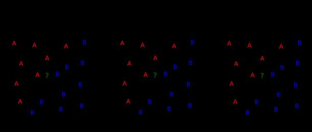
 1 Triangular points: sqrt(x 12 +x 22 ) > 0.")
41 41 Underfitting and Overfitting (Example) 500 circular and 500 triangular data points. Circular points: 0.5 sqrt(x 12 +x 22 ) 1 Triangular points: sqrt(x 12 +x 22 ) > 0.5 or sqrt(x 12 +x 22 ) < 1
42 42 Underfitting and Overfitting Overfitting Underfitting: when model is too simple, both training and test errors are large
43 43 Overfitting due to Noise Decision boundary is distorted by noise point
44 44 Notes on Overfitting Overfitting results in decision trees that are more complex than necessary Training error no longer provides a good estimate of how well the tree will perform on previously unseen records Need new ways for estimating errors
45 45 Lab4 Decision Tree
46 46 Lab4 Try different -Maximal depth - Confidence - Apply pruning / prepruning
47 47 Instance Based Classifiers Examples: Rote-learner Memorizes entire training data and performs classification only if attributes of record match one of the training examples exactly K-Nearest neighbor Uses k closest points (nearest neighbors) for performing classification
48 48 Nearest Neighbor Classifiers Basic idea: If it walks like a duck, quacks like a duck, then it s probably a duck Compute Distance Test Record Training Records Choose k of the nearest records
49 49 Nearest-Neighbor Classifiers Unknown record Requires three things The set of stored records Distance Metric to compute distance between records The value of k, the number of nearest neighbors to retrieve To classify an unknown record: Compute distance to other training records Identify k nearest neighbors Use class labels of nearest neighbors to determine the class label of unknown record (e.g., by taking majority vote)
50 50 Definition of Nearest Neighbor X X X (a) 1-nearest neighbor (b) 2-nearest neighbor (c) 3-nearest neighbor K-nearest neighbors of a record x are data points that have the k smallest distance to x
51 51 Nearest Neighbor Classification Compute distance between two points: Euclidean distance d( p, q) i ( p q i i ) 2 Determine the class from nearest neighbor list take the majority vote of class labels among the k-nearest neighbors Weigh the vote according to distance weight factor, w = 1/d 2
52 52 Nearest Neighbor Classification Choosing the value of k: If k is too small, sensitive to noise points If k is too large, neighborhood may include points from other classes X
53 53 Scaling issues Nearest Neighbor Classification Attributes may have to be scaled to prevent distance measures from being dominated by one of the attributes Example: height of a person may vary from 1.5m to 1.8m weight of a person may vary from 90lb to 300lb income of a person may vary from $10K to $1M
54 54 Nearest neighbor Classification k-nn classifiers are lazy learners It does not build models explicitly Unlike eager learners such as decision tree induction and rule-based systems Classifying unknown records are relatively expensive

55 55 55
![56 Bayes s rule Probability of event H given evidence E : Pr[ H E] Pr[ E H ]Pr[ H ] Pr[ E] A priori probability of H : Probability of event before evidence is seen A](/docs-images/93/111991538/images/56-4.jpg "posteriori probability of H : Pr[H ] Pr[ H E] Probability of event after evidence is seen Thomas Bayes Born: 1702 in London, England Died: 1761 in Tunbridge Wells, Kent,")
56 56 Bayes s rule Probability of event H given evidence E : Pr[ H E] Pr[ E H ]Pr[ H ] Pr[ E] A priori probability of H : Probability of event before evidence is seen A posteriori probability of H : Pr[H ] Pr[ H E] Probability of event after evidence is seen Thomas Bayes Born: 1702 in London, England Died: 1761 in Tunbridge Wells, Kent, England
57 57 Naïve Bayes for classification Classification learning: what s the probability of the class given an instance? Evidence E = instance Event H = class value for instance Naïve assumption: evidence splits into parts (i.e. attributes) that are independent Pr[H E] Pr[E H]Pr[E H]K Pr[E H]Pr[H] 1 2 n Pr[E]
58 58 Outlook Temp Humidity Windy Play Sunny Hot High False No Sunny Hot High True No Overcast Hot High False Yes Rainy Mild High False Yes Rainy Cool Normal False Yes Rainy Cool Normal True No Probabilities for weather data Overcast Cool Normal True Yes Sunny Mild High False No Sunny Cool Normal False Yes Rainy Mild Normal False Yes Sunny Mild Normal True Yes Overcast Mild High True Yes Overcast Hot Normal False Yes Rainy Mild High True No Outlook Temperature Humidity Windy Play Yes No Yes No Yes No Yes No Yes No Sunny 2 3 Hot 2 2 High 3 4 False Overcast 4 0 Mild 4 2 Normal 6 1 True 3 3 Rainy 3 2 Cool 3 1 Sunny 2/9 3/5 Hot 2/9 2/5 High 3/9 4/5 False 6/9 2/5 9/1 4 Overcast 4/9 0/5 Mild 4/9 2/5 Normal 6/9 1/5 True 3/9 3/5 Rainy 3/9 2/5 Cool 3/9 1/5 5/1 4
59 59 Probabilities for weather data Outlook Temperature Humidity Windy Play Yes No Yes No Yes No Yes No Yes No Sunny 2 3 Hot 2 2 High 3 4 False Overcast 4 0 Mild 4 2 Normal 6 1 True 3 3 Rainy 3 2 Cool 3 1 Sunny 2/9 3/5 Hot 2/9 2/5 High 3/9 4/5 False 6/9 2/5 9/14 5/14 Overcast 4/9 0/5 Mild 4/9 2/5 Normal 6/9 1/5 True 3/9 3/5 Rainy 3/9 2/5 Cool 3/9 1/5 A new day: Likelihood of the two classes For yes = 2/9 3/9 3/9 3/9 9/14 = Outlook Temp. Humidity Windy Play For no = 3/5 1/5 4/5 3/5 5/14 = Sunny Cool High True? Conversion into a probability by normalization: P( yes ) = / ( ) = P( no ) = / ( ) = 0.795
 The probability density function for the")
 n 1 i 1 Then the density function f(x) is f ( x ) 1 2 2 ( x)")
60 60 Numeric attributes Usual assumption: attributes have a normal or Gaussian probability distribution (given the class) The probability density function for the normal distribution is defined by two parameters: Sample mean n 1 n i 1 x i Standard deviation n 1 2 ( x i ) n 1 i 1 Then the density function f(x) is f ( x ) ( x) e

61 61 Statistics for weather data Outlook Temperature Humidity Windy Play Yes No Yes No Yes No Yes No Yes No Sunny , 68, 65, 71, 65, 70, 70, 85, False Overcast , 70, 72, 80, 70, 75, 90, 91, True 3 3 Rainy , 85, 80, 95, Sunny 2/9 3/5 =73 =75 =79 =86 False 6/9 2/5 9/14 5/14 Overcast 4/9 0/5 =6.2 =7.9 =10.2 =9.7 True 3/9 3/5 Rainy 3/9 2/5 Example density value: f ( temperature 66 yes) e (66 73)
62 62 Classifying a new day A new day: Outlook Temp. Humidity Windy Play Sunny true? Likelihood of yes = 2/ /9 9/14 = Likelihood of no = 3/ /5 5/14 = P( yes ) = / ( ) = 20.9% P( no ) = / ( ) = 79.1% Missing values during training are not included in calculation of mean and standard deviation
63 63 Naïve Bayes: discussion Naïve Bayes works surprisingly well (even if independence assumption is clearly violated) Why? Because classification doesn t require accurate probability estimates as long as maximum probability is assigned to correct class However: adding too many redundant attributes will cause problems (e.g. identical attributes) Note also: many numeric attributes are not normally distributed
64 64 Lab5 Decision Tree, Naïve Bayes, and k-nearest Neighbors

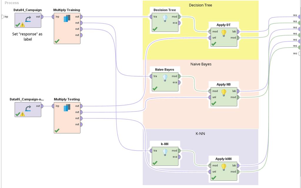
65 65 Use this operator if you want to uses the output more than once
66 66
67 67 Lab6 Decision Tree, Naïve Bayes, and k- Nearest Neighbors with Sub Processes
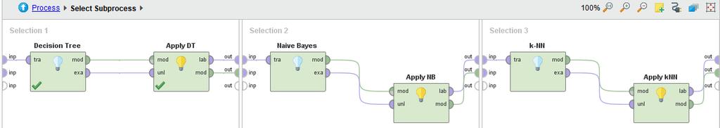
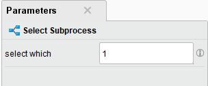
68 68 Use this operators to group some operator in one block Use this operators to select subprocesses (like switch-case)
69 69
70 70
71 71
72 72 Module 9 Classification Evaluation Techniques
73 73 Issues in evaluation Statistical reliability of estimated differences in performance ( significance tests) Choice of performance measure: Number of correct classifications Accuracy of probability estimates Error in numeric predictions Costs assigned to different types of errors Many practical applications involve costs
74 74 Training and testing I Natural performance measure for classification problems: error rate Success: instance s class is predicted correctly Error: instance s class is predicted incorrectly Error rate: proportion of errors made over the whole set of instances Resubstitution error: error rate obtained from training data Resubstitution error is (hopelessly) optimistic!
75 75 Training and testing II Test set: independent instances that have played no part in formation of classifier Assumption: both training data and test data are representative samples of the underlying problem Test and training data may differ in nature Example: classifiers built using customer data from two different towns A and B To estimate performance of classifier from town A in completely new town, test it on data from B
76 76 Note on parameter tuning It is important that the test data is not used in any way to create the classifier Some learning schemes operate in two stages: Stage 1: build the basic structure Stage 2: optimize parameter settings The test data can t be used for parameter tuning! Proper procedure uses three sets: training data, validation data, and test data Validation data is used to optimize parameters
77 77 Making the most of the data Once evaluation is complete, all the data can be used to build the final classifier Generally, the larger the training data the better the classifier (but returns diminish) The larger the test data the more accurate the error estimate Holdout procedure: method of splitting original data into training and test set Dilemma: ideally both training set and test set should be large!
78 78 Holdout estimation What to do if the amount of data is limited? The holdout method reserves a certain amount for testing and uses the remainder for training Usually: one third for testing, the rest for training Problem: the samples might not be representative Example: class might be missing in the test data Advanced version uses stratification Ensures that each class is represented with approximately equal proportions in both subsets
79 79 Repeated holdout method Holdout estimate can be made more reliable by repeating the process with different subsamples In each iteration, a certain proportion is randomly selected for training (possibly with stratificiation) The error rates on the different iterations are averaged to yield an overall error rate This is called the repeated holdout method Still not optimum: the different test sets overlap Can we prevent overlapping?
80 80 Cross-validation Cross-validation avoids overlapping test sets First step: split data into k subsets of equal size Second step: use each subset in turn for testing, the remainder for training Called k-fold cross-validation Often the subsets are stratified before the cross-validation is performed The error estimates are averaged to yield an overall error estimate
81 81 More on cross-validation Standard method for evaluation: stratified ten-fold cross-validation Why ten? Extensive experiments have shown that this is the best choice to get an accurate estimate There is also some theoretical evidence for this Stratification reduces the estimate s variance Even better: repeated stratified cross-validation E.g. ten-fold cross-validation is repeated ten times and results are averaged (reduces the variance)
82 82

83 83 Stratified 10-fold CV Round 1 Round 2 Round 3 Round 4 Round 10
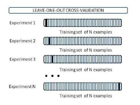
84 84 Leave-One-Out cross-validation Leave-One-Out: a particular form of cross-validation: Set number of folds to number of training instances I.e., for n training instances, build classifier n times Makes best use of the data Involves no random subsampling Very computationally expensive (exception: NN)
85 85
86 86 Metrics for Performance Evaluation Confusion Matrix: PREDICTED CLASS Class=Yes Class=No ACTUAL CLASS Class=Yes TP FN Class=No FP TN TP = True Positive TN = True Negative FP = False Positive (Type I Error) FN = False Negative (Type II Error)
87 87 Metrics for Performance Evaluation Confusion Matrix: PREDICTED CLASS Class=Yes Class=No ACTUAL CLASS Class=Yes TP FN Class=No FP TN (all correctly classified) Accuracy = all instances = TP+TN all
88 88 Limitation of Accuracy Consider a 2-class problem Number of Class 0 examples = 9990 Number of Class 1 examples = 10 If model predicts everything to be class 0, accuracy is 9990/10000 = 99.9 % Accuracy is misleading because model does not detect any class 1 example
89 89 Cost Matrix PREDICTED CLASS C(i j) Class=Yes Class=No ACTUAL CLASS Class=Yes C(Yes Yes) C(No Yes) Class=No C(Yes No) C(No No) C(i j): Cost of misclassifying class j example as class i
90 90 Computing Cost of Classification Cost Matrix ACTUAL CLASS PREDICTED CLASS C(i j) Model M 1 PREDICTED CLASS Model M 2 PREDICTED CLASS ACTUAL CLASS ACTUAL CLASS Accuracy = 80% Cost = 3910 Accuracy = 90% Cost = 4255
91 91 Metrics for Performance Evaluation Confusion Matrix: PREDICTED CLASS Class=Yes Class=No ACTUAL CLASS Class=Yes TP FN Class=No FP TN True Positive Rate (TPR)= Sensitivity = TP TP+FN
92 92 Metrics for Performance Evaluation Confusion Matrix: PREDICTED CLASS Class=Yes Class=No ACTUAL CLASS Class=Yes TP FN Class=No FP TN False positive rate (FPR)= Fall-out = FP TN+FP
93 93 Metrics for Performance Evaluation Confusion Matrix: PREDICTED CLASS Class=Yes Class=No ACTUAL CLASS Class=Yes TP FN Class=No FP TN False negative rate (FNR)= Miss Rate = FN TP+FN
94 94 Metrics for Performance Evaluation Confusion Matrix: PREDICTED CLASS Class=Yes Class=No ACTUAL CLASS Class=Yes TP FN Class=No FP TN True Negative Rate (TNR) = Specificity (SPC) = TN FN+TN
95 95 Measures in information retrieval Percentage of retrieved documents that are relevant: precision=tp/(tp+fn) Percentage of relevant documents that are returned: recall =TP/(TP+FP) Precision/recall curves have hyperbolic shape Summary measures: average precision at 20%, 50% and 80% recall (three-point average recall) F-measure=(2 recall precision)/(recall+precision)
96 96 Metrics for Performance Evaluation Confusion Matrix: PREDICTED CLASS Class=Yes Class=No ACTUAL CLASS Class=Yes TP FN Class=No FP TN Precision= TP TP+FN
97 97 Metrics for Performance Evaluation Confusion Matrix: PREDICTED CLASS Class=Yes Class=No ACTUAL CLASS Class=Yes TP FN Class=No FP TN Recall = TP TP+FP
98 98 Metrics for Performance Evaluation Confusion Matrix: PREDICTED CLASS Class=Yes Class=No ACTUAL CLASS Class=Yes TP FN Class=No FP TN F-Measure= 2 Precision Recall Precision+ Recall = 2 TP 2 TP+FP+FN
99 99 Methods for Performance Evaluation How to obtain a reliable estimate of performance? Performance of a model may depend on other factors besides the learning algorithm: Class distribution Cost of misclassification Size of training and test sets
100 100 ROC curves Stands for receiver operating characteristic Used in signal detection to show tradeoff between hit rate and false alarm rate over noisy channel y axis shows percentage of true positives in sample rather than absolute number x axis shows percentage of false positives in samplerather than sample size
101 101 ROC Curve (TP,FP): (0,0): declare everything to be negative class (1,1): declare everything to be positive class (1,0): ideal Diagonal line: Random guessing Below diagonal line: prediction is opposite of the true class
102 102 How to Construct an ROC curve Instance P(+ A) True Class Use classifier that produces posterior probability for each test instance P(+ A) Sort the instances according to P(+ A) in decreasing order Apply threshold at each unique value of P(+ A) Count the number of TP, FP, TN, FN at each threshold TP rate, TPR = TP/(TP+FN) FP rate, FPR = FP/(FP + TN)
103 103 How to construct an ROC curve Class TP FP TN FN TPR FPR ROC Curve:
104 104 ROC for one Classifier Good separation between the classes, convex curve.
105 105 ROC for one Classifier Reasonable separation between the classes, mostly convex.
106 106 ROC for one Classifier Fairly poor separation between the classes, mostly convex.
107 107 ROC for one Classifier Poor separation between the classes, large and small concavities.
108 108 ROC for one Classifier Random performance.
109 True Positive Rate True Positive Rate True Positive Rate True Positive Rate 109 AUC for ROC curves 100% 100% AUC = 100% AUC = 50% 0 % 0 % False Positive Rate 100 % 0 % 0 % False Positive Rate 100 % 100% 100% AUC = 90% AUC = 65% 0 % 0 % False Positive Rate 100 % 0 % 0 % False Positive Rate 100 %
110 110 Interpretation of AUC AUC can be interpreted as the probability that the test result from a randomly chosen diseased individual is more indicative of disease than that from a randomly chosen nondiseased individual: P(X i X j D i = 1, D j = 0) So can think of this as a nonparametric distance between disease/nondisease test results
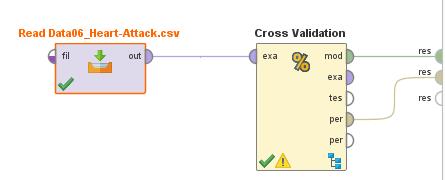
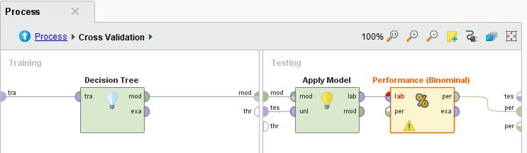
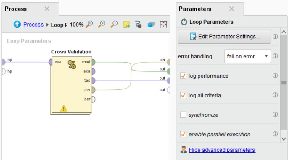
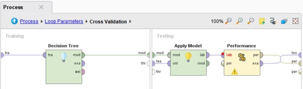
111 111 Lab7 Decision Tree with 10-Fold Cross Validation
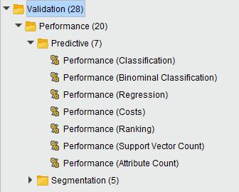

112 112 Validation
113 113
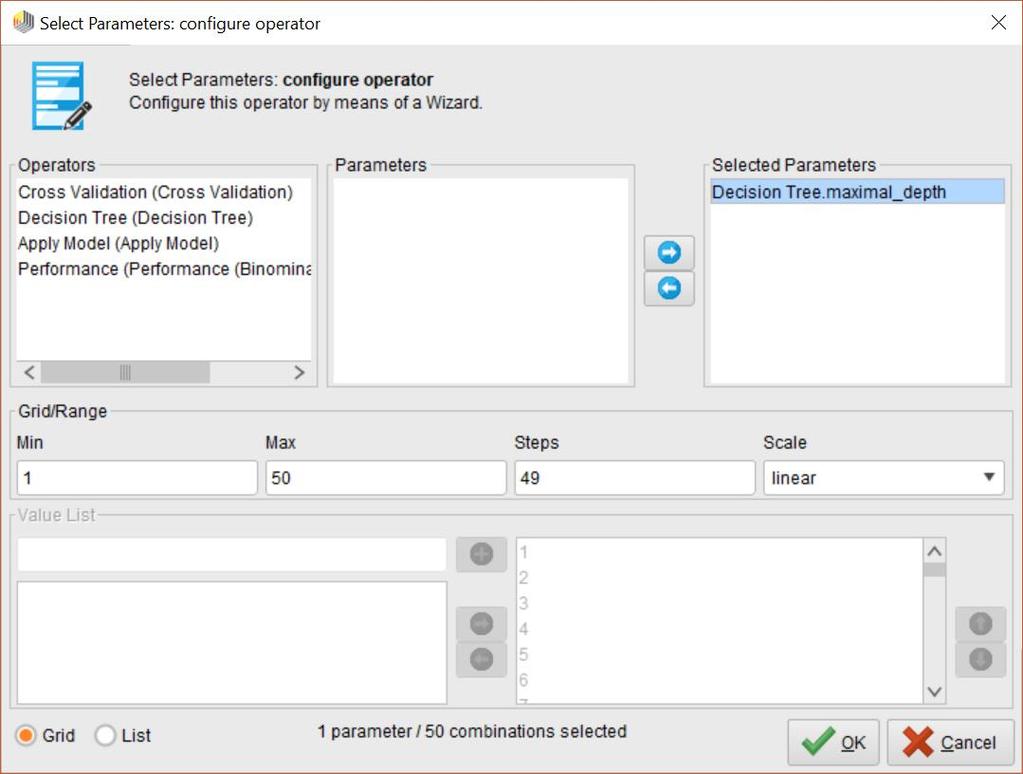
114 114 Lab8 Decision Tree with Parameters Looping

115 115 You can iterate everything


116 116 You can keep log in tabular format

117 117 Set Heart_attack as a label
118 118

119 119
120 120
121 121 Run
122 122 Module 10 Regression
123 123 Regression For classification the output(s) is nominal In regression the output is continuous Function Approximation Many models could be used Simplest is linear regression Fit data with the best hyper-plane which "goes through" the points For each point the differences between the predicted point and the actual observation is the residue y x
124 124 Simple Linear Regression For now, assume just one (input) independent variable x, and one (output) dependent variable y Multiple linear regression assumes an input vector x Multivariate linear regression assumes an output vector y We will "fit" the points with a line (i.e. hyper-plane) Which line should we use? Choose an objective function For simple linear regression we choose sum squared error (SSE) S (predicted i actual i ) 2 = S (residue i ) 2 Thus, find the line which minimizes the sum of the squared residues (e.g. least squares)
125 125 How do we "learn" parameters For the 2-d problem (line) there are coefficients for the bias and the independent variable (y-intercept and slope) Y = b 0 + b 1 X To find the values for the coefficients which minimize the objective function we take the partial derivates of the objective function (SSE) with respect to the coefficients. Set these to 0, and solve. b 1 = n å xy -åxå y nåx 2 - ( åx) 2 b 0 = åy - b 1 n å x
126 126 Multiple Linear Regression Y X X n X n There is a closed form for finding multiple linear regression weights which requires matrix inversion, etc. There are also iterative techniques to find weights One is the delta rule. For regression we use an output node which is not thresholded (just does a linear sum) and iteratively apply the delta rule thus the net is the output 2 2 Dw i = c(t -net)x i Where c is the learning rate and x is input for that weight Delta rule will update towards the objective of minimizing the SSE, thus solving multiple linear regression There are many other regression approaches that give different results by trying to better handle outliers and other statistical anomalies
127 127 SSE and Linear Regression SSE chooses to square the difference of the predicted vs actual. Why square? Don't want residues to cancel each other Could use absolute or other distances to solve problem S predicted i actual i : L1 vs L2 SSE leads to a parabolic error surface which is good for gradient descent Which line would least squares choose? There is always one best fit
128 128 SSE and Linear Regression SSE chooses to square the difference of the predicted vs actual. Why square? Don't want residues to cancel each other Could use absolute or other distances to solve problem S predicted i actual i : SSE leads to a parabolic error surface which is good for gradient descent Which line would least squares choose? There is always one best fit 7
129 129 SSE and Linear Regression SSE chooses to square the difference of the predicted vs actual. Why square? Don't want residues to cancel each other Could use absolute or other distances to solve problem S predicted i actual i : SSE leads to a parabolic error surface which is good for gradient descent Which line would least squares choose? There is always one best fit 5 7
130 130 SSE and Linear Regression SSE chooses to square the difference of the predicted vs actual. Why square? Don't want residues to cancel each other Could use absolute or other distances to solve problem S predicted i actual i : SSE leads to a parabolic error surface which is good for gradient descent Which line would least squares choose? There is always one best fit Note that the squared error causes the model to be more highly influenced by outliers Though best fit assuming Gaussian noise error from true surface
131 131 SSE and Linear Regression Generalization In generalization all x values map to a y value on the chosen regression line y Input Value x Input Value
132 132 Non-Linear Tasks Linear Regression will not generalize well to the task below Needs a non-linear surface Could do a feature pre-process as with the quadric machine For example, we could use an arbitrary polynomial in x Thus it is still linear in the coefficients, and can be solved with delta rule, etc. What order polynomial should we use? Overfit issues occur as we'll discuss later Y = b 0 + b 1 X + b 2 X b n X n
133 133 Evaluating numeric prediction Same strategies: independent test set, cross-validation, significance tests, etc. Difference: error measures Actual target values: a 1 a 2 a n Predicted target values: p 1 p 2 p n Most popular measure: mean-squared error Easy to manipulate mathematically n) ( p a1)... ( pn a n
134 134 Other measures The root mean-squared error : n) ( p a1)... ( pn a n The mean absolute error is less sensitive to outliers than the meansquared error: p a1... n Sometimes relative error values are more appropriate (e.g. 10% for an error of 50 when predicting 500) p 1 n an
135 135 Improvement on the mean How much does the scheme improve on simply predicting the average? The relative squared error is ( ): The relative absolute error is: ) (... ) ( ) (... ) ( n n n a a a a a p a p the average a is n n n a a a a a p a p
136 136 Correlation coefficient Measures the statistical correlation between the predicted values and the actual values Scale independent, between 1 and +1 Good performance leads to large values! A P PA S S S 1 ) )( ( n a a p p S i i i PA 1 ) ( 2 n p p S i i P 1 ) ( 2 n a a S i i A
137 137 Correlation coefficient
138 138 Which measure? Best to look at all of them Often it doesn t matter Example: A B C D Root mean-squared error Mean absolute error Root rel squared error 42.2% 57.2% 39.4% 35.8% Relative absolute error 43.1% 40.1% 34.8% 30.4% Correlation coefficient D best C second-best A, B arguable
139 139 Lab9 Linear Regression

140 140 Retrieve Data08_wine
141 141

142 142
143 143 Module 11 Advanced Classification Techniques

144 144 Neural Networks What is a Neural Network? Biologically motivated approach to machine learning Similarity with biological network Fundamental processing elements of a neural network is a neuron 1.Receives inputs from other source 2.Combines them in someway 3.Performs a generally nonlinear operation on the result 4.Outputs the final result
145 145 Neural Network Neural Network is a set of connected INPUT/OUTPUT UNITS, where each connection has a WEIGHT associated with it. Neural Network learning is also called CONNECTIONIST learning due to the connections between units. It is a case of SUPERVISED, INDUCTIVE or CLASSIFICATION learning.
146 146 Neural Network Neural Network learns by adjusting the weights so as to be able to correctly classify the training data and hence, after testing phase, to classify unknown data. Neural Network needs long time for training. Neural Network has a high tolerance to noisy and incomplete data
147 147 One Neuron as a Network Here x1 and x2 are normalized attribute value of data. y is the output of the neuron, i.e the class label. x1 and x2 values multiplied by weight values w1 and w2 are input to the neuron x. Value of x1 is multiplied by a weight w1 and values of x2 is multiplied by a weight w2. Given that w1 = 0.5 and w2 = 0.5 Say value of x1 is 0.3 and value of x2 is 0.8, So, weighted sum is : sum= w1 x x1 + w2 x x2 = 0.5 x x 0.8 = 0.55
148 148 Bias of a Neuron We need the bias value to be added to the weighted sum wixi so that we can transform it from the origin. v = wixi + b, here b is the bias x2 x1-x2= -1 x1-x2=0 x1-x2= 1 x1
149 149 Bias as extra input Input Attribute values x 0 = +1 x 1 x 2 x m w 0 W1 w 2 w m weights v Activation function ( ) Summing function v m wjx j Output class y w 0 j 0 b
150 150 Neuron with Activation The neuron is the basic information processing unit of a NN. It consists of: 1 A set of links, describing the neuron inputs, with weights W 1, W 2,, W m 2. An adder function (linear combiner) for computing the weighted sum of the inputs (real numbers): u m wjxj j 1 3 Activation function : for limiting the amplitude of the neuron output. y (u b)

151 151 Activation Function
152 152 Multi-layer 152
153 153 Why We Need Multi Layer? Linear Separable: x y x y Linear inseparable: Solution? x y
154 154 Why We Need Multi Layer? False True f : >=1? Output Layer S w1 = 1 w2 = 1 OR function x1 x2 Input Layer
155 155 Why We Need Multi Layer? f : >=1? S False True Output Layer w1 = 0.5 w2 = 0.5 AND function x1 x2 Input Layer
156 156 Why We Need Multi Layer? f : >=1? False True Output Layer S w = 1 w = 1 f : >=1? f : >=1? XOR function S S Hidden Layer w = -1 w = -1 x1 w = 1 w = 1 x2 Input Layer
157 157 A Multilayer Feed-Forward Neural Output Class O k Output nodes Network O j Hidden nodes w jk w ij - weights Input nodes Input Record : x i Network is fully connected
158 158 Classification by Back propagation Back Propagation learns by iteratively processing a set of training data (samples). For each sample, weights are modified to minimize the error between network s classification and actual classification.
159 159 Steps in Back propagation Algorithm STEP ONE: initialize the weights and biases. The weights in the network are initialized to random numbers from the interval [-1,1]. Each unit has a BIAS associated with it The biases are similarly initialized to random numbers from the interval [-1,1]. STEP TWO: feed the training sample.
160 160 Steps in Back propagation Algorithm ( cont..) STEP THREE: Propagate the inputs forward; we compute the net input and output of each unit in the hidden and output layers. STEP FOUR: back propagate the error. STEP FIVE: update weights and biases to reflect the propagated errors. STEP SIX: terminating conditions.
161 161 Terminating Conditions All w ij in the previous epoch are below some threshold, or The percentage of samples misclassified in the previous epoch is below some threshold, or a pre specified number of epochs has expired. In practice, several hundreds of thousands of epochs may be required before the weights will converge.

162 162 Artificial Neural Network
163 163 Artificial Neural Network
164 164 Training Process of the MLP The training will be continued until the RMS is minimized. ERROR Local Minimum W (N dimensional) Global Minimum Local Minimum
165 165 Back prop requires many epochs to converge Some ideas to overcome this Stochastic learning Faster Convergence Update weights after each training example Momentum Add fraction of previous update to current update Faster convergence
166 166 Advantages of ANN Able to deal with (identify/model) highly nonlinear relationships Not prone to restricting normality and/or independence assumptions Can handle variety of problem types Usually provides better results (prediction and/or clustering) compared to its statistical counterparts Handles both numerical and categorical variables (transformation needed!)
167 167 Disadvantages of ANN They are deemed to be black-box solutions, lacking expandability It is hard to find optimal values for large number of network parameters Optimal design is still an art: requires expertise and extensive experimentation It is hard to handle large number of variables (especially the rich nominal attributes) Training may take a long time for large datasets; which may require case sampling
168 168 Remember.. ANNs perform well, generally better with larger number of hidden units More hidden units generally produce lower error Determining network topology is difficult Choosing single learning rate impossible Difficult to reduce training time by altering the network topology or learning parameters NN(Subset) often produce better results
169 169 Lab10 Neural Network with 10-fold Cross Validation

170 170 Retrieve Data08_Car


171 171 Input hidden layer Layer Name: H1 Size: 6

172 172 Random Tree The Random Tree learns decision trees from both nominal and numerical data. Decision trees are powerful classification methods which can be easily understood. The Random Tree operator works similar to Quinlan's C4.5 or CART but it selects a random subset of attributes before it is applied. The size of the subset is specified by the subset ratio parameter.
173 173

174 174 Random Forest The Random Forest operator generates a set of random trees. The random trees are generated in exactly the same way as the Random Tree operator generates a tree.
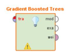
175 175 Gradient Boosted Trees
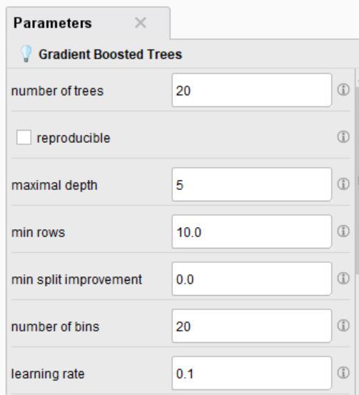
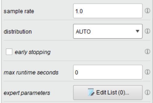
176 176
177 177 Lab11 All about trees
178 178
179 179 Try evaluating them
180 180
181 181 Optimization To find the optimal values of the selected parameters for the Operators in its subprocess.
 Find the optimal values for a set of parameters using a quadratic interaction model.")
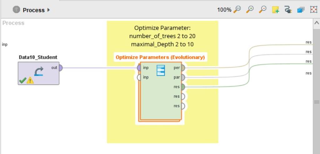
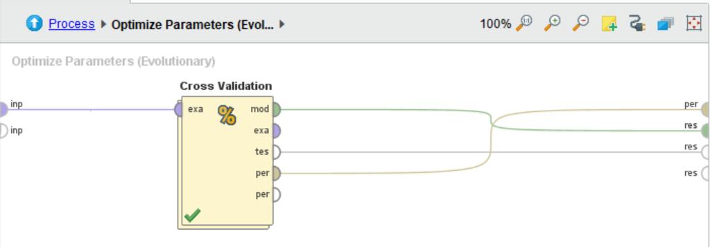
182 182 Optimization Optimize Parameters (Grid) Executes the subprocess for all combinations of selected values of the parameters and then delivers the optimal parameter values. Optimize Parameters (Quadratic) Find the optimal values for a set of parameters using a quadratic interaction model. Optimize Parameters (Evolutionary) Find the optimal values for a set of parameters using an evolutionary approach often more appropriate than a grid search (as in the Optimize Parameters (Grid) operator) or a greedy search (as in the Optimize Parameters (Quadratic) operator) and leads to better results.
183 183 Lab12 Parameter Optimization
184 184

185 185
186 186 Lab13 Prescriptive Analytics

187 187 class name = computer
188 188 Module 12 Model Integration and Results Optimization
189 189 Ensemble Methods Construct a set of classifiers from the training data Predict class label of previously unseen records by aggregating predictions made by multiple classifiers
190 190 General Idea D Original Training data Step 1: Create Multiple Data Sets... D 1 D 2 D t-1 D t Step 2: Build Multiple Classifiers C 1 C 2 C t -1 C t Step 3: Combine Classifiers C *
191 191 Why does it work? Suppose there are 25 base classifiers Each classifier has error rate, = 0.35 Assume classifiers are independent Probability that the ensemble classifier makes a wrong prediction: 25 i i (1 ) i 25 i 0.06
192 192 Examples of Ensemble Methods How to generate an ensemble of classifiers? Bagging Boosting
193 193 Bagging Sampling with replacement Original Data Bagging (Round 1) Bagging (Round 2) Bagging (Round 3) Build classifier on each bootstrap sample Each sample has probability (1 1/n) n of being selected
194 194 Boosting An iterative procedure to adaptively change distribution of training data by focusing more on previously misclassified records Initially, all N records are assigned equal weights Unlike bagging, weights may change at the end of boosting round
195 195 Boosting Records that are wrongly classified will have their weights increased Records that are classified correctly will have their weights decreased Original Data Boosting (Round 1) Boosting (Round 2) Boosting (Round 3) Example 4 is hard to classify Its weight is increased, therefore it is more likely to be chosen again in subsequent rounds
196 196 RapidMiner: Bagging and Boosting Put multiple classifiers inside one this operator Put one classifier inside one of these operators
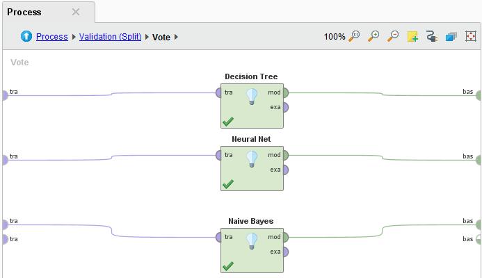
197 197 Lab14 Voting
198 198
199 199


200 200 Some of other useful operators Convert Trees to Rules Real-time output simulator Group any kinds of models to a single model sequentially Create Mathematical formulas from such model

201
Classification and Regression
 Classification and Regression Announcements Study guide for exam is on the LMS Sample exam will be posted by Monday Reminder that phase 3 oral presentations are being held next week during workshops Plan
DATA MINING LECTURE 11. Classification Basic Concepts Decision Trees Evaluation Nearest-Neighbor Classifier
 DATA MINING LECTURE 11 Classification Basic Concepts Decision Trees Evaluation Nearest-Neighbor Classifier What is a hipster? Examples of hipster look A hipster is defined by facial hair Hipster or Hippie?
Classification: Basic Concepts, Decision Trees, and Model Evaluation
 Classification: Basic Concepts, Decision Trees, and Model Evaluation Data Warehousing and Mining Lecture 4 by Hossen Asiful Mustafa Classification: Definition Given a collection of records (training set
Data Mining Concepts & Techniques
 Data Mining Concepts & Techniques Lecture No. 03 Data Processing, Data Mining Naeem Ahmed Email: naeemmahoto@gmail.com Department of Software Engineering Mehran Univeristy of Engineering and Technology
Data Mining Classification: Basic Concepts, Decision Trees, and Model Evaluation. Lecture Notes for Chapter 4. Introduction to Data Mining
 Data Mining Classification: Basic Concepts, Decision Trees, and Model Evaluation Lecture Notes for Chapter 4 Introduction to Data Mining by Tan, Steinbach, Kumar (modified by Predrag Radivojac, 2017) Classification:
DATA MINING LECTURE 9. Classification Basic Concepts Decision Trees Evaluation
 DATA MINING LECTURE 9 Classification Basic Concepts Decision Trees Evaluation What is a hipster? Examples of hipster look A hipster is defined by facial hair Hipster or Hippie? Facial hair alone is not
CSE4334/5334 DATA MINING
 CSE4334/5334 DATA MINING Lecture 4: Classification (1) CSE4334/5334 Data Mining, Fall 2014 Department of Computer Science and Engineering, University of Texas at Arlington Chengkai Li (Slides courtesy
DATA MINING LECTURE 9. Classification Decision Trees Evaluation
 DATA MINING LECTURE 9 Classification Decision Trees Evaluation 10 10 Illustrating Classification Task Tid Attrib1 Attrib2 Attrib3 Class 1 Yes Large 125K No 2 No Medium 100K No 3 No Small 70K No 4 Yes Medium
Data Mining Classification: Basic Concepts, Decision Trees, and Model Evaluation. Lecture Notes for Chapter 4. Introduction to Data Mining
 Data Mining Classification: Basic Concepts, Decision Trees, and Model Evaluation Lecture Notes for Chapter 4 Introduction to Data Mining by Tan, Steinbach, Kumar Tan,Steinbach, Kumar Introduction to Data
CS Machine Learning
 CS 60050 Machine Learning Decision Tree Classifier Slides taken from course materials of Tan, Steinbach, Kumar 10 10 Illustrating Classification Task Tid Attrib1 Attrib2 Attrib3 Class 1 Yes Large 125K
Classification. Instructor: Wei Ding
 Classification Part II Instructor: Wei Ding Tan,Steinbach, Kumar Introduction to Data Mining 4/18/004 1 Practical Issues of Classification Underfitting and Overfitting Missing Values Costs of Classification
DATA MINING LECTURE 10B. Classification k-nearest neighbor classifier Naïve Bayes Logistic Regression Support Vector Machines
 DATA MINING LECTURE 10B Classification k-nearest neighbor classifier Naïve Bayes Logistic Regression Support Vector Machines NEAREST NEIGHBOR CLASSIFICATION 10 10 Illustrating Classification Task Tid Attrib1
Naïve Bayes Classification. Material borrowed from Jonathan Huang and I. H. Witten s and E. Frank s Data Mining and Jeremy Wyatt and others
 Naïve Bayes Classification Material borrowed from Jonathan Huang and I. H. Witten s and E. Frank s Data Mining and Jeremy Wyatt and others Things We d Like to Do Spam Classification Given an email, predict
10 Classification: Evaluation
 CSE4334/5334 Data Mining 10 Classification: Evaluation Chengkai Li Department of Computer Science and Engineering University of Texas at Arlington Fall 2018 (Slides courtesy of Pang-Ning Tan, Michael Steinbach
Machine Learning. Decision Trees. Le Song /15-781, Spring Lecture 6, September 6, 2012 Based on slides from Eric Xing, CMU
 Machine Learning 10-701/15-781, Spring 2008 Decision Trees Le Song Lecture 6, September 6, 2012 Based on slides from Eric Xing, CMU Reading: Chap. 1.6, CB & Chap 3, TM Learning non-linear functions f:
Classification Part 4
 Classification Part 4 Dr. Sanjay Ranka Professor Computer and Information Science and Engineering University of Florida, Gainesville Model Evaluation Metrics for Performance Evaluation How to evaluate
Machine Learning Techniques for Data Mining
 Machine Learning Techniques for Data Mining Eibe Frank University of Waikato New Zealand 10/25/2000 1 PART V Credibility: Evaluating what s been learned 10/25/2000 2 Evaluation: the key to success How
Part I. Instructor: Wei Ding
 Classification Part I Instructor: Wei Ding Tan,Steinbach, Kumar Introduction to Data Mining 4/18/2004 1 Classification: Definition Given a collection of records (training set ) Each record contains a set
Metrics for Performance Evaluation How to evaluate the performance of a model? Methods for Performance Evaluation How to obtain reliable estimates?
 Model Evaluation Metrics for Performance Evaluation How to evaluate the performance of a model? Methods for Performance Evaluation How to obtain reliable estimates? Methods for Model Comparison How to
CS 584 Data Mining. Classification 3
 CS 584 Data Mining Classification 3 Today Model evaluation & related concepts Additional classifiers Naïve Bayes classifier Support Vector Machine Ensemble methods 2 Model Evaluation Metrics for Performance
Naïve Bayes Classification. Material borrowed from Jonathan Huang and I. H. Witten s and E. Frank s Data Mining and Jeremy Wyatt and others
 Naïve Bayes Classification Material borrowed from Jonathan Huang and I. H. Witten s and E. Frank s Data Mining and Jeremy Wyatt and others Things We d Like to Do Spam Classification Given an email, predict
Classification Salvatore Orlando
 Classification Salvatore Orlando 1 Classification: Definition Given a collection of records (training set ) Each record contains a set of attributes, one of the attributes is the class. The values of the
Machine Learning and Bioinformatics 機器學習與生物資訊學
 Molecular Biomedical Informatics 分子生醫資訊實驗室 機器學習與生物資訊學 Machine Learning & Bioinformatics 1 Evaluation The key to success 2 Three datasets of which the answers must be known 3 Note on parameter tuning It
Data Mining Classification: Bayesian Decision Theory
 Data Mining Classification: Bayesian Decision Theory Lecture Notes for Chapter 2 R. O. Duda, P. E. Hart, and D. G. Stork, Pattern classification, 2nd ed. New York: Wiley, 2001. Lecture Notes for Chapter
Lecture Notes for Chapter 4
 Classification - Basic Concepts, Decision Trees, and Model Evaluation Lecture Notes for Chapter 4 Slides by Tan, Steinbach, Kumar adapted by Michael Hahsler Look for accompanying R code on the course web
Example of DT Apply Model Example Learn Model Hunt s Alg. Measures of Node Impurity DT Examples and Characteristics. Classification.
 lassification-decision Trees, Slide 1/56 Classification Decision Trees Huiping Cao lassification-decision Trees, Slide 2/56 Examples of a Decision Tree Tid Refund Marital Status Taxable Income Cheat 1
CSE 5243 INTRO. TO DATA MINING
 CSE 5243 INTRO. TO DATA MINING Classification (Basic Concepts) Huan Sun, CSE@The Ohio State University 09/12/2017 Slides adapted from UIUC CS412, Fall 2017, by Prof. Jiawei Han Classification: Basic Concepts
CS4491/CS 7265 BIG DATA ANALYTICS
 CS4491/CS 7265 BIG DATA ANALYTICS EVALUATION * Some contents are adapted from Dr. Hung Huang and Dr. Chengkai Li at UT Arlington Dr. Mingon Kang Computer Science, Kennesaw State University Evaluation for
Extra readings beyond the lecture slides are important:
 1 Notes To preview next lecture: Check the lecture notes, if slides are not available: http://web.cse.ohio-state.edu/~sun.397/courses/au2017/cse5243-new.html Check UIUC course on the same topic. All their
Classification. Instructor: Wei Ding
 Classification Decision Tree Instructor: Wei Ding Tan,Steinbach, Kumar Introduction to Data Mining 4/18/2004 1 Preliminaries Each data record is characterized by a tuple (x, y), where x is the attribute
Part I. Classification & Decision Trees. Classification. Classification. Week 4 Based in part on slides from textbook, slides of Susan Holmes
 Week 4 Based in part on slides from textbook, slides of Susan Holmes Part I Classification & Decision Trees October 19, 2012 1 / 1 2 / 1 Classification Classification Problem description We are given a
Data Mining Classification - Part 1 -
 Data Mining Classification - Part 1 - Universität Mannheim Bizer: Data Mining I FSS2019 (Version: 20.2.2018) Slide 1 Outline 1. What is Classification? 2. K-Nearest-Neighbors 3. Decision Trees 4. Model
Evaluation Measures. Sebastian Pölsterl. April 28, Computer Aided Medical Procedures Technische Universität München
 Evaluation Measures Sebastian Pölsterl Computer Aided Medical Procedures Technische Universität München April 28, 2015 Outline 1 Classification 1. Confusion Matrix 2. Receiver operating characteristics
LECTURE NOTES Professor Anita Wasilewska NEURAL NETWORKS
 LECTURE NOTES Professor Anita Wasilewska NEURAL NETWORKS Neural Networks Classifier Introduction INPUT: classification data, i.e. it contains an classification (class) attribute. WE also say that the class
Network Traffic Measurements and Analysis
 DEIB - Politecnico di Milano Fall, 2017 Sources Hastie, Tibshirani, Friedman: The Elements of Statistical Learning James, Witten, Hastie, Tibshirani: An Introduction to Statistical Learning Andrew Ng:
Data Mining. Practical Machine Learning Tools and Techniques. Slides for Chapter 5 of Data Mining by I. H. Witten, E. Frank and M. A.
 Data Mining Practical Machine Learning Tools and Techniques Slides for Chapter 5 of Data Mining by I. H. Witten, E. Frank and M. A. Hall Credibility: Evaluating what s been learned Issues: training, testing,
Data Mining D E C I S I O N T R E E. Matteo Golfarelli
 Data Mining D E C I S I O N T R E E Matteo Golfarelli Decision Tree It is one of the most widely used classification techniques that allows you to represent a set of classification rules with a tree. Tree:
Data Mining Classification: Alternative Techniques. Imbalanced Class Problem
 Data Mining Classification: Alternative Techniques Imbalanced Class Problem Introduction to Data Mining, 2 nd Edition by Tan, Steinbach, Karpatne, Kumar Class Imbalance Problem Lots of classification problems
CS 584 Data Mining. Classification 1
 CS 584 Data Mining Classification 1 Classification: Definition Given a collection of records (training set ) Each record contains a set of attributes, one of the attributes is the class. Find a model for
9 Classification: KNN and SVM
 CSE4334/5334 Data Mining 9 Classification: KNN and SVM Chengkai Li Department of Computer Science and Engineering University of Texas at Arlington Fall 2017 (Slides courtesy of Pang-Ning Tan, Michael Steinbach
Data Mining Algorithms: Basic Methods
 Algorithms: The basic methods Inferring rudimentary rules Data Mining Algorithms: Basic Methods Chapter 4 of Data Mining Statistical modeling Constructing decision trees Constructing rules Association
CLASSIFICATION WITH RADIAL BASIS AND PROBABILISTIC NEURAL NETWORKS
 CLASSIFICATION WITH RADIAL BASIS AND PROBABILISTIC NEURAL NETWORKS CHAPTER 4 CLASSIFICATION WITH RADIAL BASIS AND PROBABILISTIC NEURAL NETWORKS 4.1 Introduction Optical character recognition is one of
BBS654 Data Mining. Pinar Duygulu. Slides are adapted from Nazli Ikizler
 BBS654 Data Mining Pinar Duygulu Slides are adapted from Nazli Ikizler 1 Classification: Basic Concepts Classification: Basic Concepts Decision Tree Induction Bayes Classification Methods Model Evaluation
Weka ( )
") Weka ( http://www.cs.waikato.ac.nz/ml/weka/ ) The phases in which classifier s design can be divided are reflected in WEKA s Explorer structure: Data pre-processing (filtering) and representation Supervised
Weka ( http://www.cs.waikato.ac.nz/ml/weka/ ) The phases in which classifier s design can be divided are reflected in WEKA s Explorer structure: Data pre-processing (filtering) and representation Supervised
Classification with Decision Tree Induction
 Classification with Decision Tree Induction This algorithm makes Classification Decision for a test sample with the help of tree like structure (Similar to Binary Tree OR k-ary tree) Nodes in the tree
Business Club. Decision Trees
 Business Club Decision Trees Business Club Analytics Team December 2017 Index 1. Motivation- A Case Study 2. The Trees a. What is a decision tree b. Representation 3. Regression v/s Classification 4. Building
COMPUTATIONAL INTELLIGENCE SEW (INTRODUCTION TO MACHINE LEARNING) SS18. Lecture 6: k-nn Cross-validation Regularization
 SS18. Lecture 6: k-nn Cross-validation Regularization") COMPUTATIONAL INTELLIGENCE SEW (INTRODUCTION TO MACHINE LEARNING) SS18 Lecture 6: k-nn Cross-validation Regularization LEARNING METHODS Lazy vs eager learning Eager learning generalizes training data before
COMPUTATIONAL INTELLIGENCE SEW (INTRODUCTION TO MACHINE LEARNING) SS18 Lecture 6: k-nn Cross-validation Regularization LEARNING METHODS Lazy vs eager learning Eager learning generalizes training data before
Lecture Notes for Chapter 5
 Classifcation - Alternative Techniques Lecture Notes for Chapter 5 Slides by Tan, Steinbach, Kumar adapted by Michael Hahsler Look for accompanying R code on the course web site. Topics Rule-Based Classifier
Classification Lecture Notes cse352. Neural Networks. Professor Anita Wasilewska
 Classification Lecture Notes cse352 Neural Networks Professor Anita Wasilewska Neural Networks Classification Introduction INPUT: classification data, i.e. it contains an classification (class) attribute
CS6375: Machine Learning Gautam Kunapuli. Mid-Term Review
 Gautam Kunapuli Machine Learning Data is identically and independently distributed Goal is to learn a function that maps to Data is generated using an unknown function Learn a hypothesis that minimizes
Decision Trees Dr. G. Bharadwaja Kumar VIT Chennai
 Decision Trees Decision Tree Decision Trees (DTs) are a nonparametric supervised learning method used for classification and regression. The goal is to create a model that predicts the value of a target
Slides for Data Mining by I. H. Witten and E. Frank
 Slides for Data Mining by I. H. Witten and E. Frank 7 Engineering the input and output Attribute selection Scheme-independent, scheme-specific Attribute discretization Unsupervised, supervised, error-
Data Preprocessing. Supervised Learning
 Supervised Learning Regression Given the value of an input X, the output Y belongs to the set of real values R. The goal is to predict output accurately for a new input. The predictions or outputs y are
Data Mining and Machine Learning: Techniques and Algorithms
 Instance based classification Data Mining and Machine Learning: Techniques and Algorithms Eneldo Loza Mencía eneldo@ke.tu-darmstadt.de Knowledge Engineering Group, TU Darmstadt International Week 2019,
Machine Learning Techniques for Data Mining
 Machine Learning Techniques for Data Mining Eibe Frank University of Waikato New Zealand 10/25/2000 1 PART VII Moving on: Engineering the input and output 10/25/2000 2 Applying a learner is not all Already
Classification Algorithms in Data Mining
 August 9th, 2016 Suhas Mallesh Yash Thakkar Ashok Choudhary CIS660 Data Mining and Big Data Processing -Dr. Sunnie S. Chung Classification Algorithms in Data Mining Deciding on the classification algorithms
CISC 4631 Data Mining
 CISC 4631 Data Mining Lecture 05: Overfitting Evaluation: accuracy, precision, recall, ROC Theses slides are based on the slides by Tan, Steinbach and Kumar (textbook authors) Eamonn Koegh (UC Riverside)
DATA MINING OVERFITTING AND EVALUATION
 DATA MINING OVERFITTING AND EVALUATION 1 Overfitting Will cover mechanisms for preventing overfitting in decision trees But some of the mechanisms and concepts will apply to other algorithms 2 Occam s
CS 229 Midterm Review
 CS 229 Midterm Review Course Staff Fall 2018 11/2/2018 Outline Today: SVMs Kernels Tree Ensembles EM Algorithm / Mixture Models [ Focus on building intuition, less so on solving specific problems. Ask
Pattern Recognition. Kjell Elenius. Speech, Music and Hearing KTH. March 29, 2007 Speech recognition
 Pattern Recognition Kjell Elenius Speech, Music and Hearing KTH March 29, 2007 Speech recognition 2007 1 Ch 4. Pattern Recognition 1(3) Bayes Decision Theory Minimum-Error-Rate Decision Rules Discriminant
MIT 801. Machine Learning I. [Presented by Anna Bosman] 16 February 2018
![MIT 801. Machine Learning I. [Presented by Anna Bosman] 16 February 2018](/thumbs/77/76295965.jpg "MIT 801. Machine Learning I. [Presented by Anna Bosman] 16 February 2018") MIT 801 [Presented by Anna Bosman] 16 February 2018 Machine Learning What is machine learning? Artificial Intelligence? Yes as we know it. What is intelligence? The ability to acquire and apply knowledge
MIT 801 [Presented by Anna Bosman] 16 February 2018 Machine Learning What is machine learning? Artificial Intelligence? Yes as we know it. What is intelligence? The ability to acquire and apply knowledge
Evaluating Classifiers
 Evaluating Classifiers Reading for this topic: T. Fawcett, An introduction to ROC analysis, Sections 1-4, 7 (linked from class website) Evaluating Classifiers What we want: Classifier that best predicts
Artificial Intelligence. Programming Styles
 Artificial Intelligence Intro to Machine Learning Programming Styles Standard CS: Explicitly program computer to do something Early AI: Derive a problem description (state) and use general algorithms to
Random Forest A. Fornaser
 Random Forest A. Fornaser alberto.fornaser@unitn.it Sources Lecture 15: decision trees, information theory and random forests, Dr. Richard E. Turner Trees and Random Forests, Adele Cutler, Utah State University
Analytical model A structure and process for analyzing a dataset. For example, a decision tree is a model for the classification of a dataset.
 Glossary of data mining terms: Accuracy Accuracy is an important factor in assessing the success of data mining. When applied to data, accuracy refers to the rate of correct values in the data. When applied
Information Management course
 Università degli Studi di Milano Master Degree in Computer Science Information Management course Teacher: Alberto Ceselli Lecture 20: 10/12/2015 Data Mining: Concepts and Techniques (3 rd ed.) Chapter
Data Mining and Machine Learning. Instance-Based Learning. Rote Learning k Nearest-Neighbor Classification. IBL and Rule Learning
 Data Mining and Machine Learning Instance-Based Learning Rote Learning k Nearest-Neighbor Classification Prediction, Weighted Prediction choosing k feature weighting (RELIEF) instance weighting (PEBLS)
Neural Networks. CE-725: Statistical Pattern Recognition Sharif University of Technology Spring Soleymani
 Neural Networks CE-725: Statistical Pattern Recognition Sharif University of Technology Spring 2013 Soleymani Outline Biological and artificial neural networks Feed-forward neural networks Single layer
Evaluating Classifiers
 Evaluating Classifiers Reading for this topic: T. Fawcett, An introduction to ROC analysis, Sections 1-4, 7 (linked from class website) Evaluating Classifiers What we want: Classifier that best predicts
A Systematic Overview of Data Mining Algorithms
 A Systematic Overview of Data Mining Algorithms 1 Data Mining Algorithm A well-defined procedure that takes data as input and produces output as models or patterns well-defined: precisely encoded as a
Contents Machine Learning concepts 4 Learning Algorithm 4 Predictive Model (Model) 4 Model, Classification 4 Model, Regression 4 Representation
 4 Model, Classification 4 Model, Regression 4 Representation") Contents Machine Learning concepts 4 Learning Algorithm 4 Predictive Model (Model) 4 Model, Classification 4 Model, Regression 4 Representation Learning 4 Supervised Learning 4 Unsupervised Learning 4
Contents Machine Learning concepts 4 Learning Algorithm 4 Predictive Model (Model) 4 Model, Classification 4 Model, Regression 4 Representation Learning 4 Supervised Learning 4 Unsupervised Learning 4
Data Mining and Analytics
 Data Mining and Analytics Aik Choon Tan, Ph.D. Associate Professor of Bioinformatics Division of Medical Oncology Department of Medicine aikchoon.tan@ucdenver.edu 9/22/2017 http://tanlab.ucdenver.edu/labhomepage/teaching/bsbt6111/
International Journal of Scientific Research & Engineering Trends Volume 4, Issue 6, Nov-Dec-2018, ISSN (Online): X
: X") Analysis about Classification Techniques on Categorical Data in Data Mining Assistant Professor P. Meena Department of Computer Science Adhiyaman Arts and Science College for Women Uthangarai, Krishnagiri,
Analysis about Classification Techniques on Categorical Data in Data Mining Assistant Professor P. Meena Department of Computer Science Adhiyaman Arts and Science College for Women Uthangarai, Krishnagiri,
COMP 465: Data Mining Classification Basics
 Supervised vs. Unsupervised Learning COMP 465: Data Mining Classification Basics Slides Adapted From : Jiawei Han, Micheline Kamber & Jian Pei Data Mining: Concepts and Techniques, 3 rd ed. Supervised
7. Decision or classification trees
 7. Decision or classification trees Next we are going to consider a rather different approach from those presented so far to machine learning that use one of the most common and important data structure,
Big Data Methods. Chapter 5: Machine learning. Big Data Methods, Chapter 5, Slide 1
 Big Data Methods Chapter 5: Machine learning Big Data Methods, Chapter 5, Slide 1 5.1 Introduction to machine learning What is machine learning? Concerned with the study and development of algorithms that
CS249: ADVANCED DATA MINING
 CS249: ADVANCED DATA MINING Classification Evaluation and Practical Issues Instructor: Yizhou Sun yzsun@cs.ucla.edu April 24, 2017 Homework 2 out Announcements Due May 3 rd (11:59pm) Course project proposal
The Curse of Dimensionality
 The Curse of Dimensionality ACAS 2002 p1/66 Curse of Dimensionality The basic idea of the curse of dimensionality is that high dimensional data is difficult to work with for several reasons: Adding more
INTRODUCTION TO MACHINE LEARNING. Measuring model performance or error
 INTRODUCTION TO MACHINE LEARNING Measuring model performance or error Is our model any good? Context of task Accuracy Computation time Interpretability 3 types of tasks Classification Regression Clustering
Cse634 DATA MINING TEST REVIEW. Professor Anita Wasilewska Computer Science Department Stony Brook University
 Cse634 DATA MINING TEST REVIEW Professor Anita Wasilewska Computer Science Department Stony Brook University Preprocessing stage Preprocessing: includes all the operations that have to be performed before
Chapter 3: Supervised Learning
 Chapter 3: Supervised Learning Road Map Basic concepts Evaluation of classifiers Classification using association rules Naïve Bayesian classification Naïve Bayes for text classification Summary 2 An example
Lecture outline. Decision-tree classification
 Lecture outline Decision-tree classification Decision Trees Decision tree A flow-chart-like tree structure Internal node denotes a test on an attribute Branch represents an outcome of the test Leaf nodes
ECLT 5810 Evaluation of Classification Quality
 ECLT 5810 Evaluation of Classification Quality Reference: Data Mining Practical Machine Learning Tools and Techniques, by I. Witten, E. Frank, and M. Hall, Morgan Kaufmann Testing and Error Error rate:
Applying Supervised Learning
 Applying Supervised Learning When to Consider Supervised Learning A supervised learning algorithm takes a known set of input data (the training set) and known responses to the data (output), and trains
Evaluating Machine-Learning Methods. Goals for the lecture
 Evaluating Machine-Learning Methods Mark Craven and David Page Computer Sciences 760 Spring 2018 www.biostat.wisc.edu/~craven/cs760/ Some of the slides in these lectures have been adapted/borrowed from
List of Exercises: Data Mining 1 December 12th, 2015
 List of Exercises: Data Mining 1 December 12th, 2015 1. We trained a model on a two-class balanced dataset using five-fold cross validation. One person calculated the performance of the classifier by measuring
Predictive Analytics: Demystifying Current and Emerging Methodologies. Tom Kolde, FCAS, MAAA Linda Brobeck, FCAS, MAAA
 Predictive Analytics: Demystifying Current and Emerging Methodologies Tom Kolde, FCAS, MAAA Linda Brobeck, FCAS, MAAA May 18, 2017 About the Presenters Tom Kolde, FCAS, MAAA Consulting Actuary Chicago,
Data Mining. 3.2 Decision Tree Classifier. Fall Instructor: Dr. Masoud Yaghini. Chapter 5: Decision Tree Classifier
 Data Mining 3.2 Decision Tree Classifier Fall 2008 Instructor: Dr. Masoud Yaghini Outline Introduction Basic Algorithm for Decision Tree Induction Attribute Selection Measures Information Gain Gain Ratio
Naïve Bayes for text classification
 Road Map Basic concepts Decision tree induction Evaluation of classifiers Rule induction Classification using association rules Naïve Bayesian classification Naïve Bayes for text classification Support
Nominal Data. May not have a numerical representation Distance measures might not make sense. PR and ANN
 NonMetric Data Nominal Data So far we consider patterns to be represented by feature vectors of real or integer values Easy to come up with a distance (similarity) measure by using a variety of mathematical
Data Mining and Knowledge Discovery Practice notes 2
 Keywords Data Mining and Knowledge Discovery: Practice Notes Petra Kralj Novak Petra.Kralj.Novak@ijs.si Data Attribute, example, attribute-value data, target variable, class, discretization Algorithms
Chapter 4: Algorithms CS 795
 Chapter 4: Algorithms CS 795 Inferring Rudimentary Rules 1R Single rule one level decision tree Pick each attribute and form a single level tree without overfitting and with minimal branches Pick that
Probabilistic Classifiers DWML, /27
 Probabilistic Classifiers DWML, 2007 1/27 Probabilistic Classifiers Conditional class probabilities Id. Savings Assets Income Credit risk 1 Medium High 75 Good 2 Low Low 50 Bad 3 High Medium 25 Bad 4 Medium
Nonparametric Methods Recap
 Nonparametric Methods Recap Aarti Singh Machine Learning 10-701/15-781 Oct 4, 2010 Nonparametric Methods Kernel Density estimate (also Histogram) Weighted frequency Classification - K-NN Classifier Majority
Evaluating Classifiers
 Evaluating Classifiers Charles Elkan elkan@cs.ucsd.edu January 18, 2011 In a real-world application of supervised learning, we have a training set of examples with labels, and a test set of examples with
CS570: Introduction to Data Mining
 CS570: Introduction to Data Mining Classification Advanced Reading: Chapter 8 & 9 Han, Chapters 4 & 5 Tan Anca Doloc-Mihu, Ph.D. Slides courtesy of Li Xiong, Ph.D., 2011 Han, Kamber & Pei. Data Mining.
Introduction to Machine Learning
 Introduction to Machine Learning Decision Tree Example Three variables: Attribute 1: Hair = {blond, dark} Attribute 2: Height = {tall, short} Class: Country = {Gromland, Polvia} CS4375 --- Fall 2018 a
CSC411/2515 Tutorial: K-NN and Decision Tree
 CSC411/2515 Tutorial: K-NN and Decision Tree Mengye Ren csc{411,2515}ta@cs.toronto.edu September 25, 2016 Cross-validation K-nearest-neighbours Decision Trees Review: Motivation for Validation Framework:
Representing structural patterns: Reading Material: Chapter 3 of the textbook by Witten
 Representing structural patterns: Plain Classification rules Decision Tree Rules with exceptions Relational solution Tree for Numerical Prediction Instance-based presentation Reading Material: Chapter
INTRODUCTION TO DATA MINING. Daniel Rodríguez, University of Alcalá
 INTRODUCTION TO DATA MINING Daniel Rodríguez, University of Alcalá Outline Knowledge Discovery in Datasets Model Representation Types of models Supervised Unsupervised Evaluation (Acknowledgement: Jesús